Practical mapping examples with MAFF data

Mapping MAFF data

Read data from the MAFF database 地域の農業を見て・知って・活かすDB.

library(fude)
library(ggplot2)

d <- read_fude("~/MB0001_2025_2020_38.zip", quiet = TRUE)
b1 <- get_boundary(d, path = "~", boundary_type = 1, quiet = TRUE)
m1 <- read_ikasudb(b1, "~/IA0001_2023_2020_38.xlsx")

m1$地域類型1次分類 <- factor(m1$地域類型1次分類, labels = c("都市的地域", "平地農業地域", "中間農業地域", "山間農業地域"))

ggplot() +
  geom_sf(data = m1, aes(fill = 地域類型1次分類), alpha = .8) +
  theme_void() +
  theme(text = element_text(family = "Hiragino Sans"))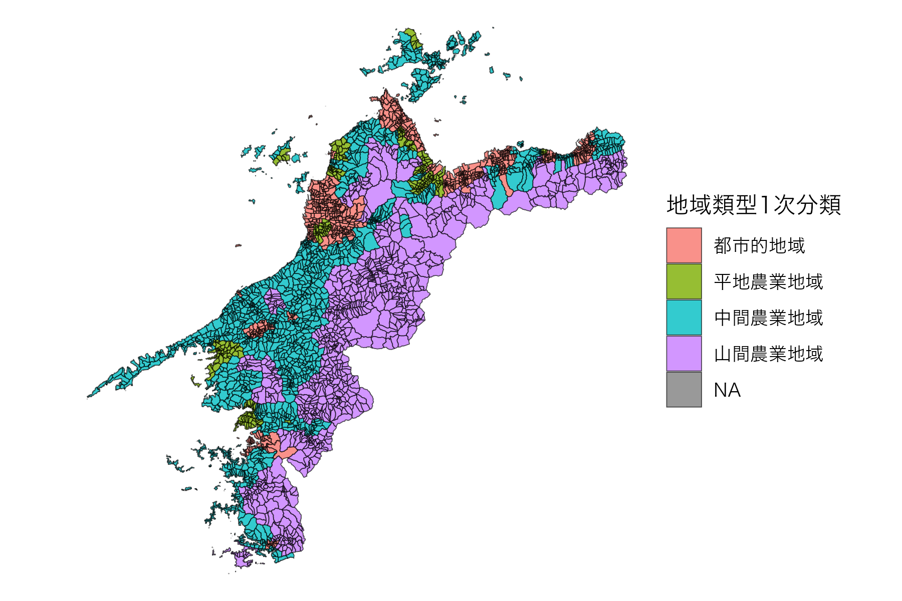

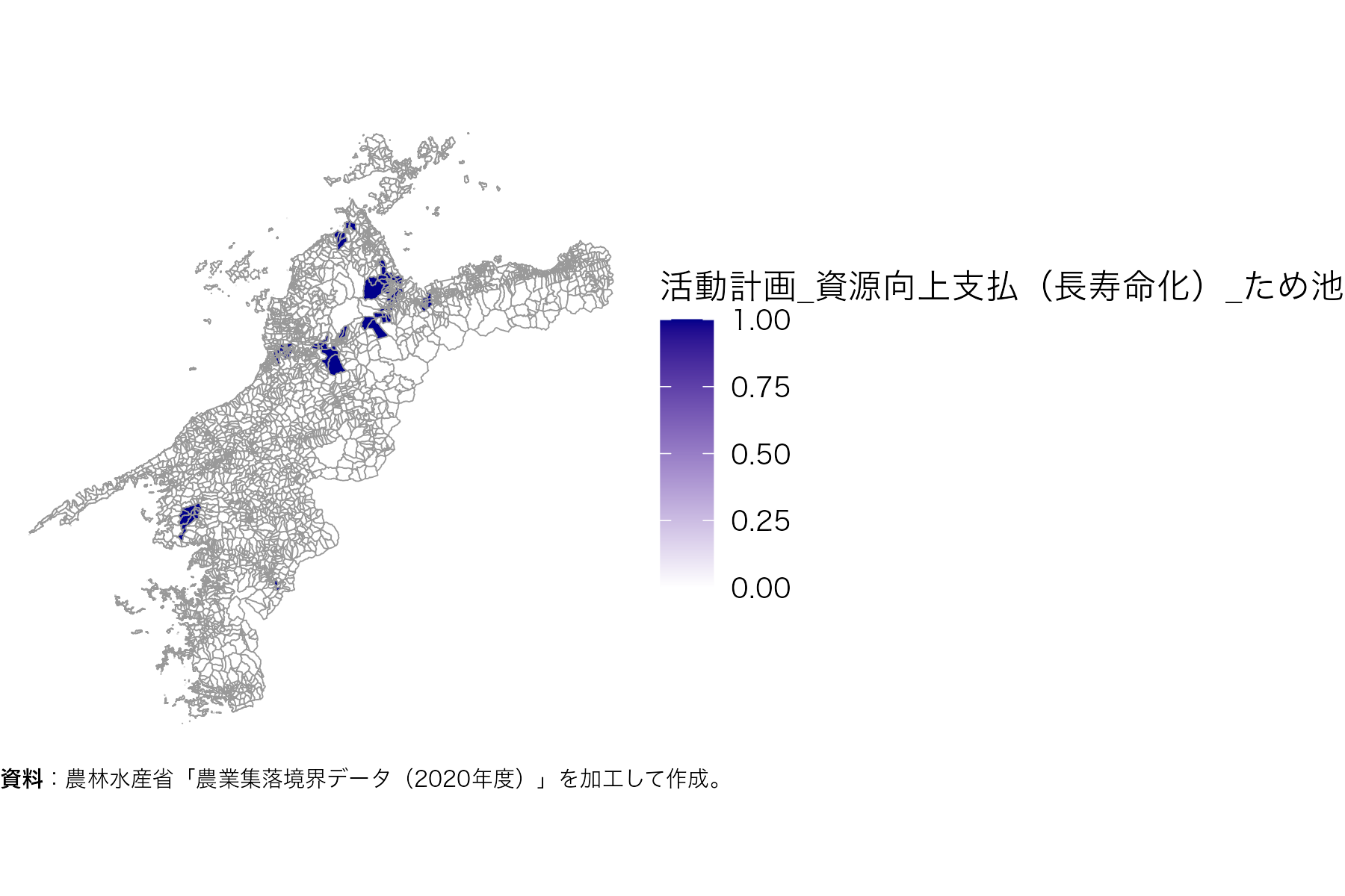
資料：農林水産省「農業集落境界データ（2020年度）」を加工して作成。

b2 <- get_boundary(d, path = "~", boundary_type = 2, quiet = TRUE)
m2 <- read_ikasudb(b2, "~/IA0001_2023_2020_38.xlsx")

m2$地域類型1次分類 <- factor(m2$地域類型1次分類, labels = c("都市的地域", "平地農業地域", "中間農業地域", "山間農業地域"))

ggplot() +
  geom_sf(data = m2, aes(fill = 地域類型1次分類), alpha = .8) +
  theme_void() +
  theme(text = element_text(family = "Hiragino Sans"))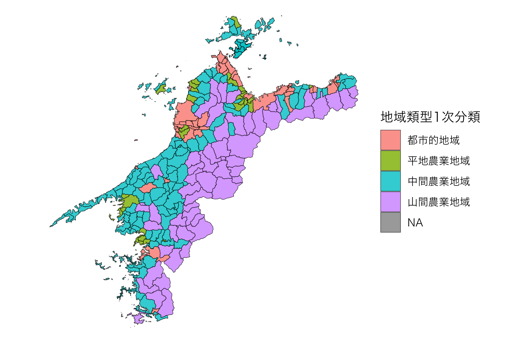

資料：農林水産省「農業集落境界データ（2020年度）」を加工して作成。

b3 <- get_boundary(d, path = "~", boundary_type = 3, quiet = TRUE)
m3 <- read_ikasudb(b3, "~/IA0001_2023_2020_38.xlsx")

m3$地域類型1次分類 <- factor(m3$地域類型1次分類, levels = 1:4, labels = c("都市的地域", "平地農業地域", "中間農業地域", "山間農業地域"))

ggplot() +
  geom_sf(data = m3, aes(fill = 地域類型1次分類), alpha = .8) +
  theme_void() +
  theme(text = element_text(family = "Hiragino Sans"))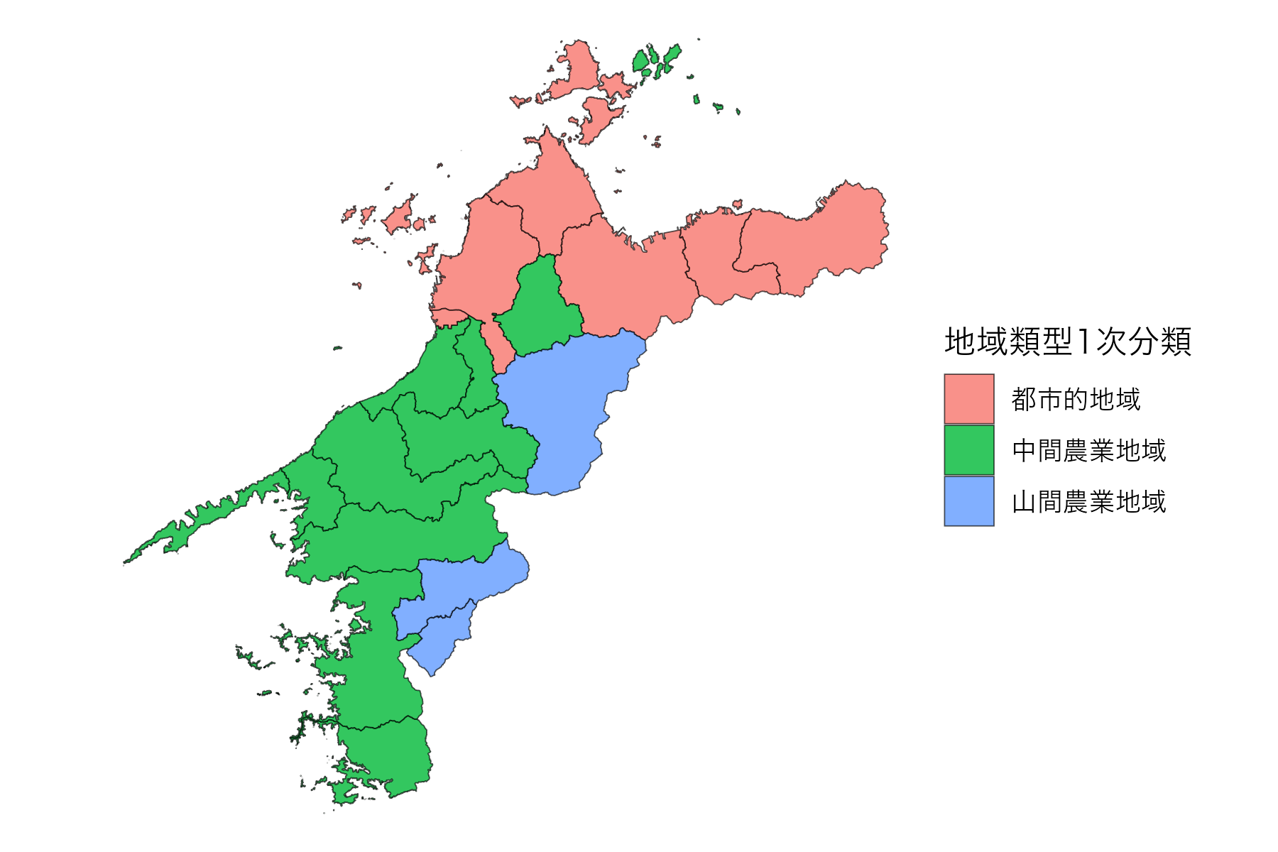

資料：農林水産省「農業集落境界データ（2020年度）」を加工して作成。

library(ggtext)

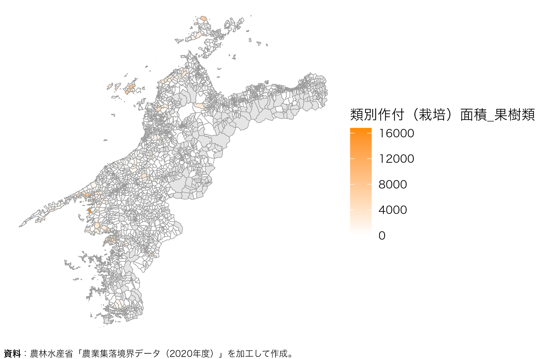
m1 <- read_ikasudb(b1, "~/SA1066_2020_2020_38.xlsx")

ggplot() +
  geom_sf(data = m1, aes(fill = `類別作付（栽培）面積_果樹類`), color = "grey60") +
  scale_fill_gradient(
    low  = "white",
    high = "darkorange",
    na.value = "grey90"
  ) +
  labs(caption = paste0("**資料**：", cite_fude(m1)$ja)) +
  theme_void() +
  theme(
    plot.caption = element_markdown(size = 7, hjust = 0),
    text = element_text(family = "Hiragino Sans")
  )

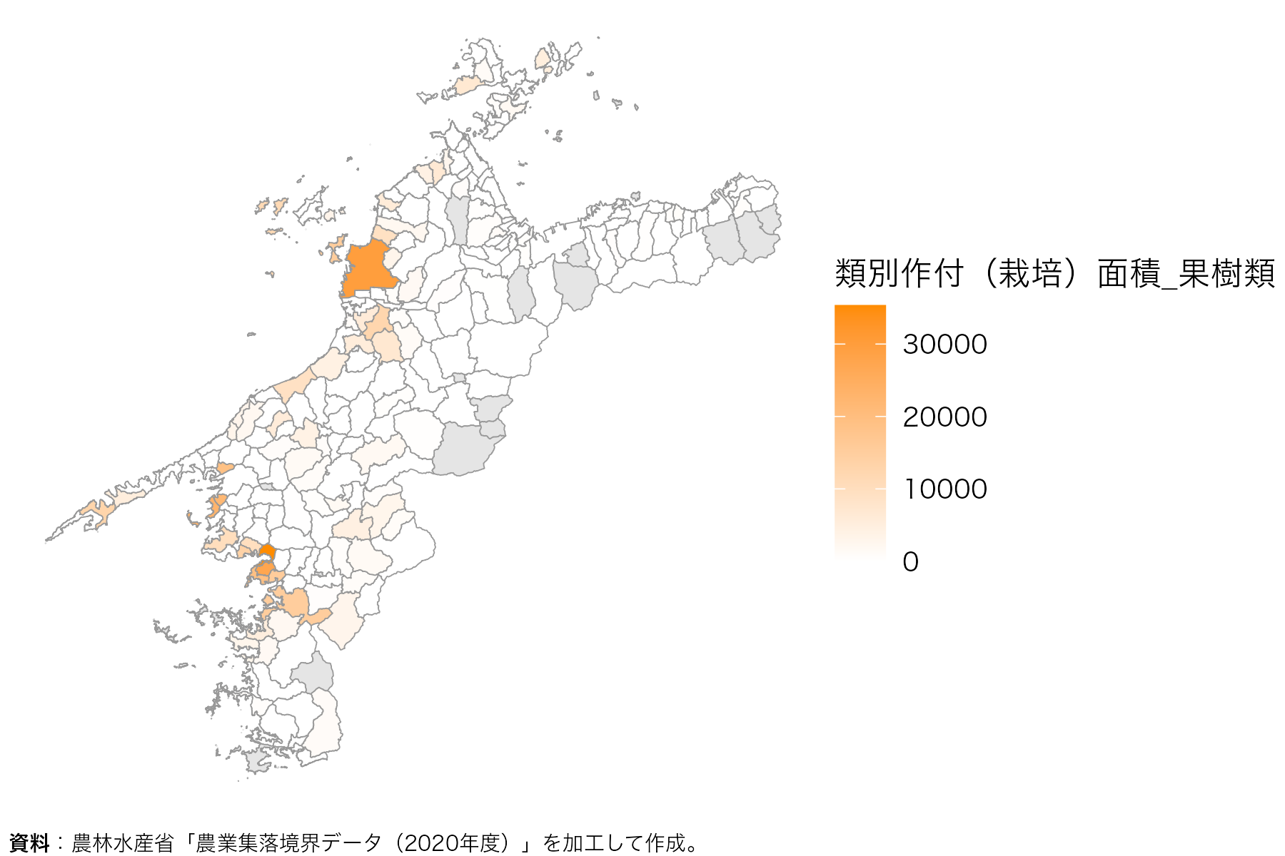
m2 <- read_ikasudb(b2, "~/SA1066_2020_2020_38.xlsx")

ggplot() +
  geom_sf(data = m2, aes(fill = `類別作付（栽培）面積_果樹類`), color = "grey60") +
  scale_fill_gradient(
    low  = "white",
    high = "darkorange",
    na.value = "grey90"
  ) +
  labs(caption = paste0("**資料**：", cite_fude(m2)$ja)) +
  theme_void() +
  theme(
    plot.caption = element_markdown(size = 7, hjust = 0),
    text = element_text(family = "Hiragino Sans")
  )

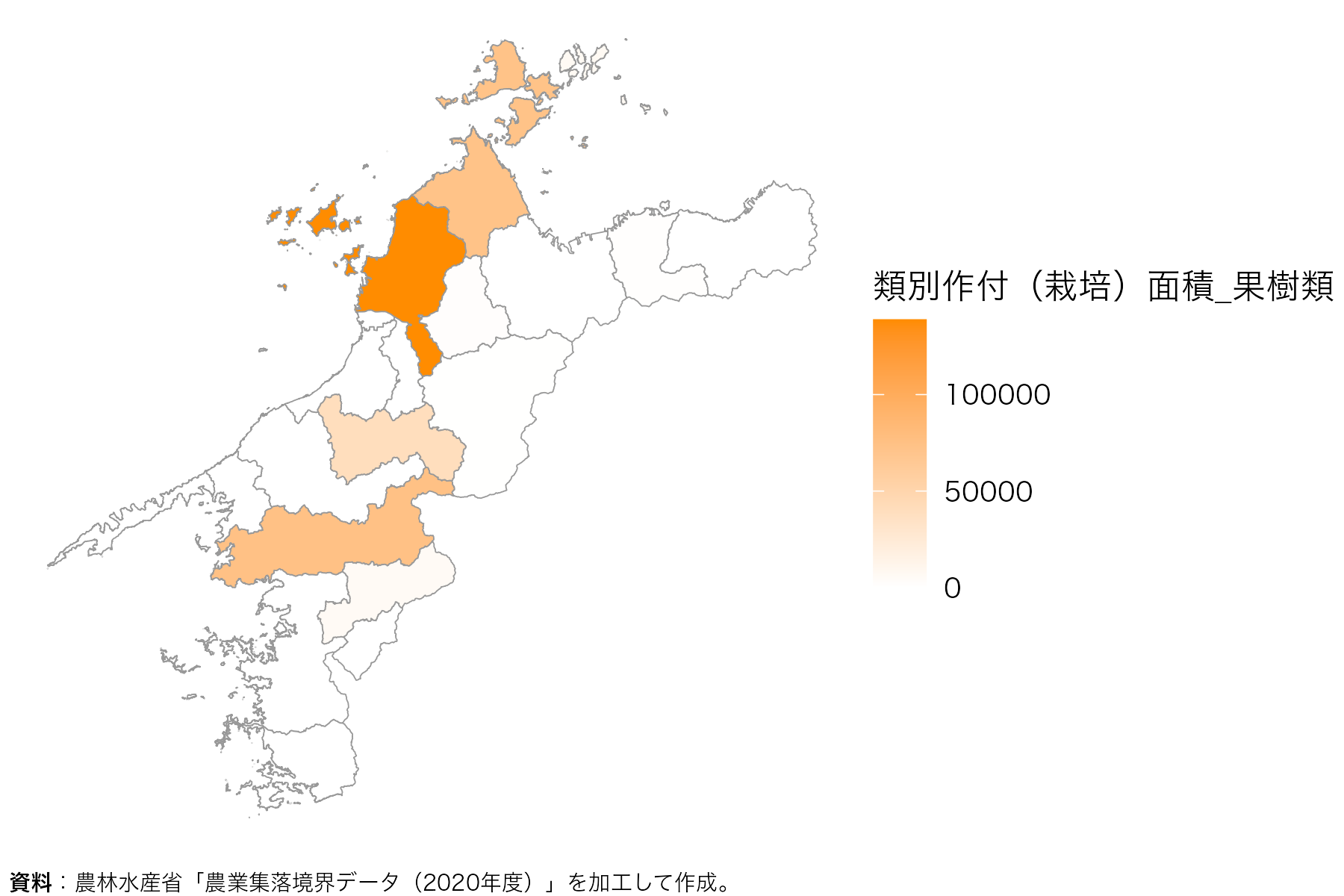
m3 <- read_ikasudb(b3, "~/SA1066_2020_2020_38.xlsx")

ggplot() +
  geom_sf(data = m3, aes(fill = `類別作付（栽培）面積_果樹類`), color = "grey60") +
  scale_fill_gradient(
    low  = "white",
    high = "darkorange",
    na.value = "grey90"
  ) +
  labs(caption = paste0("**資料**：", cite_fude(m3)$ja)) +
  theme_void() +
  theme(
    plot.caption = element_markdown(size = 7, hjust = 0),
    text = element_text(family = "Hiragino Sans")
  )

m1 <- b1 |>
  read_ikasudb("~/GC0001_2019_2020_38.xlsx")

library(mapview)

mapview(m1, zcol = "組織数")

t1 <- extract_boundary(m1, city = "東温")

mapview(t1, zcol = "組織数")

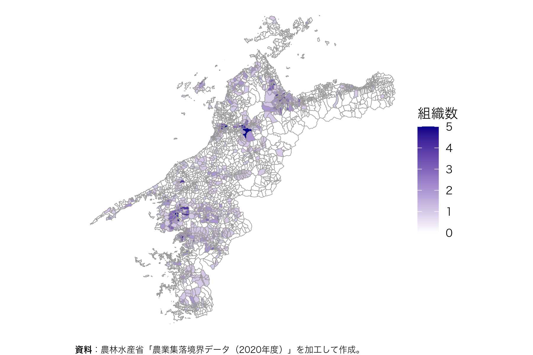
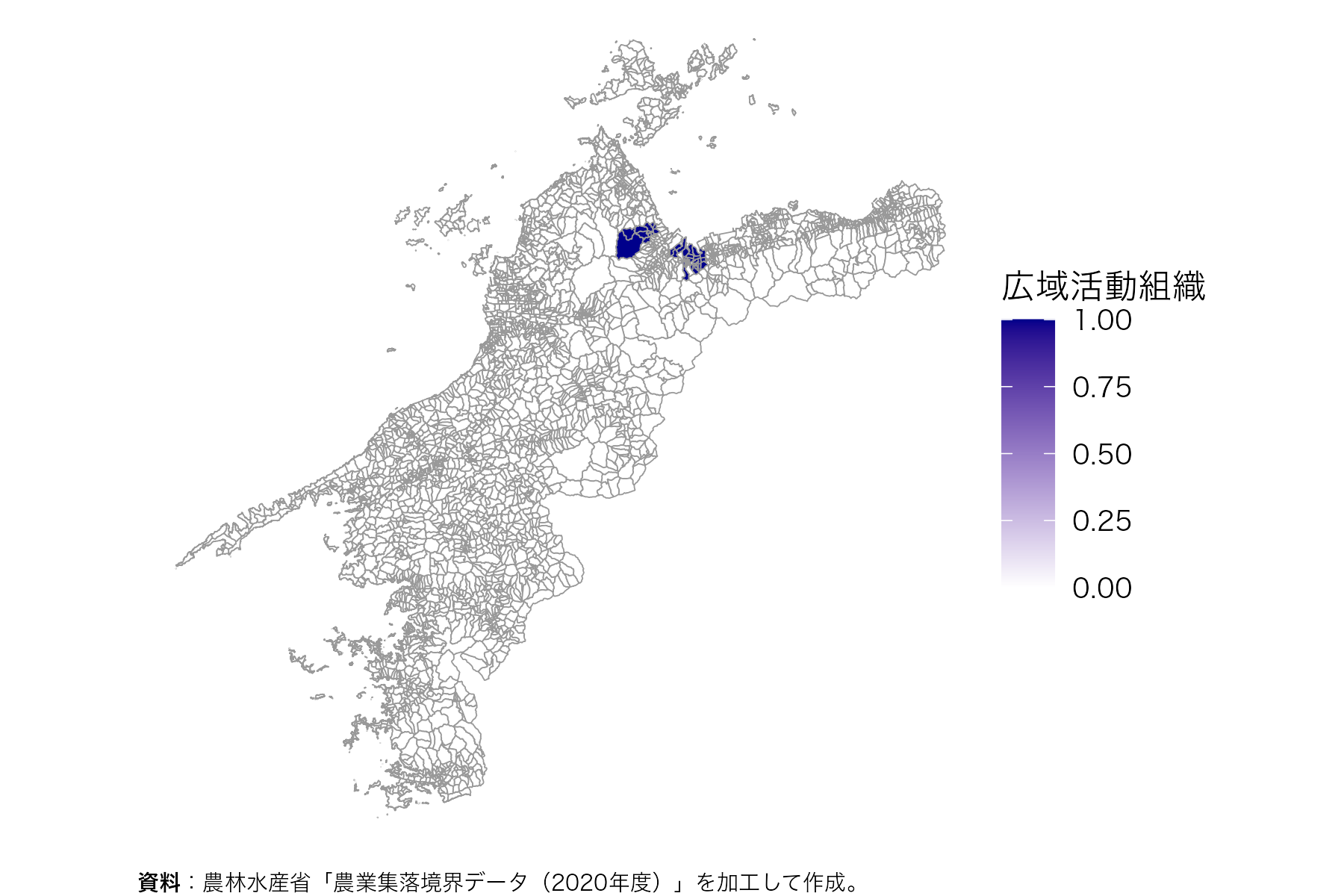
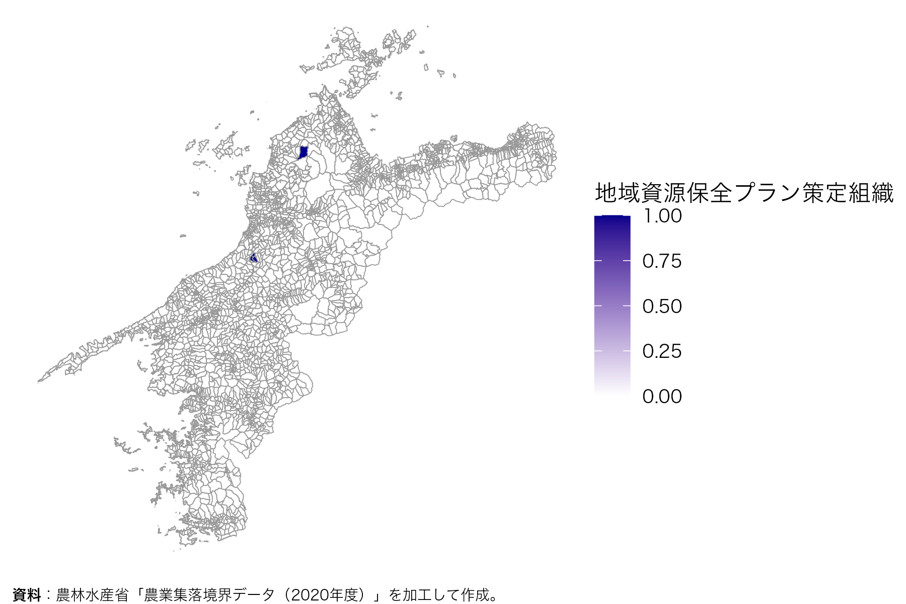
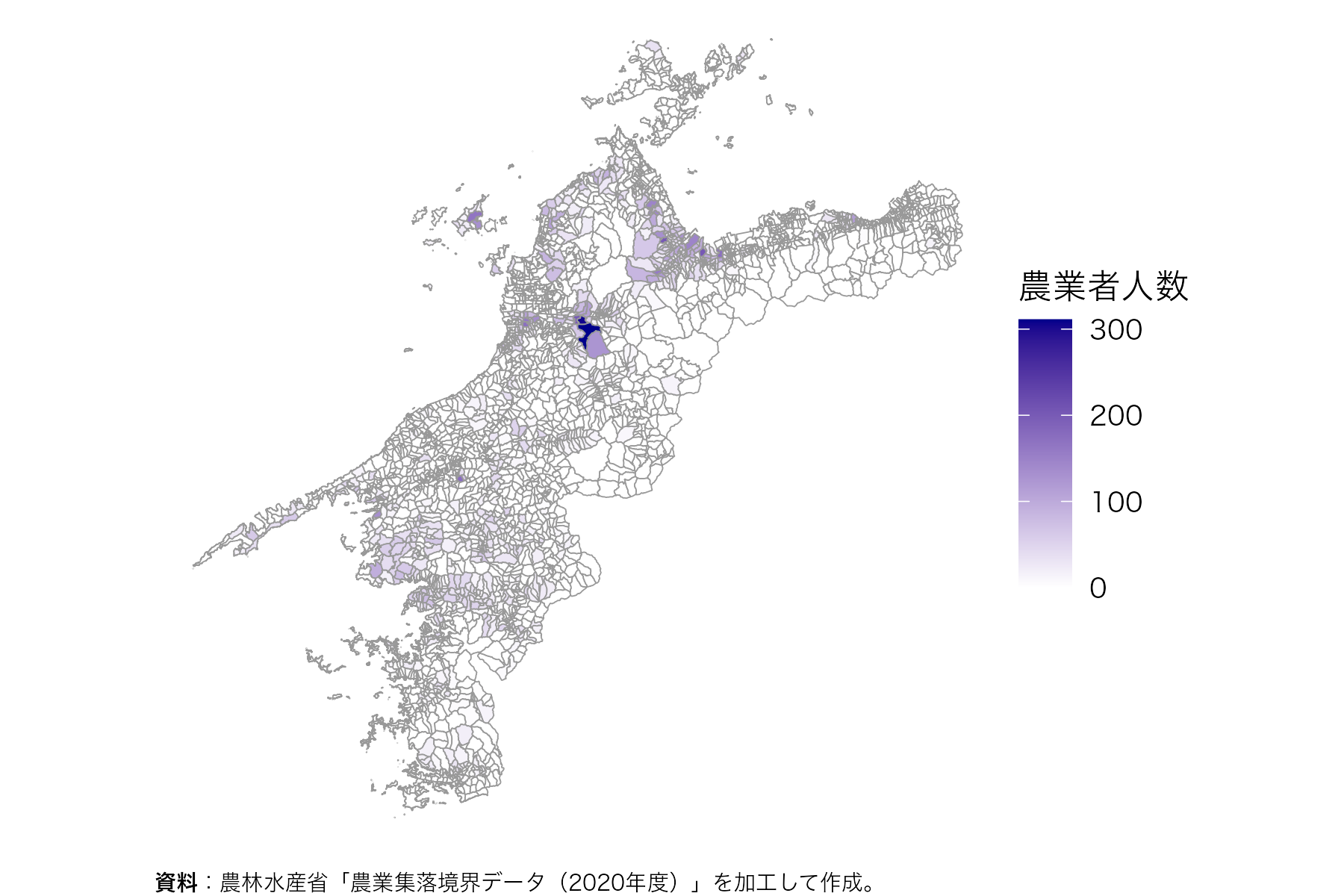
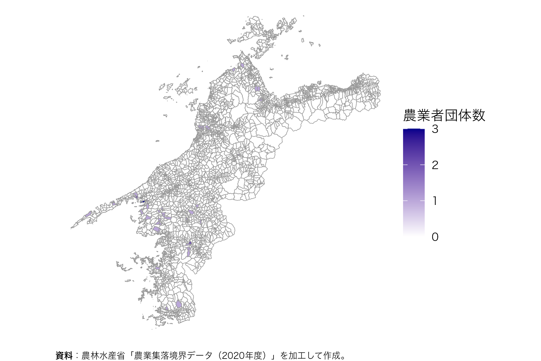
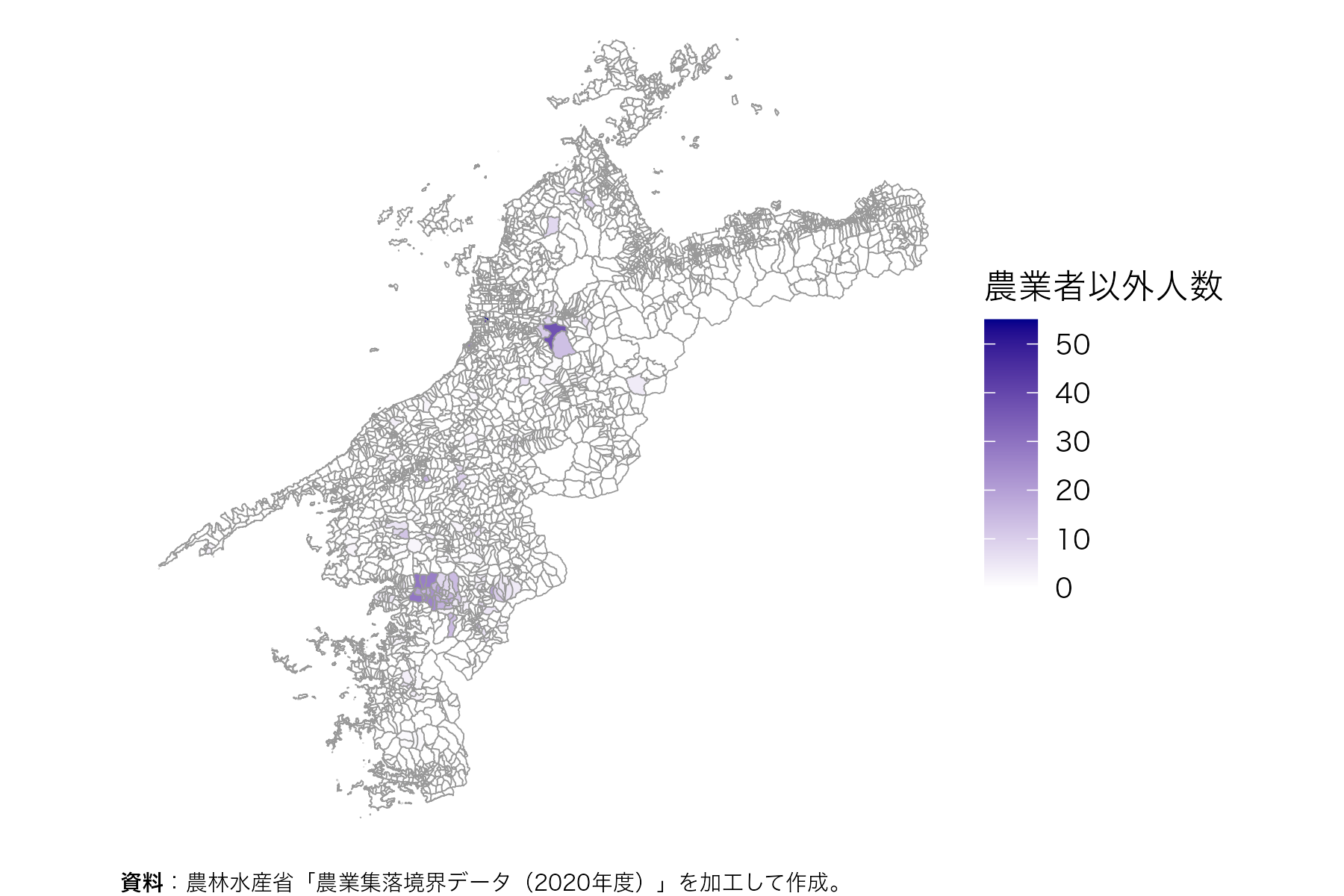
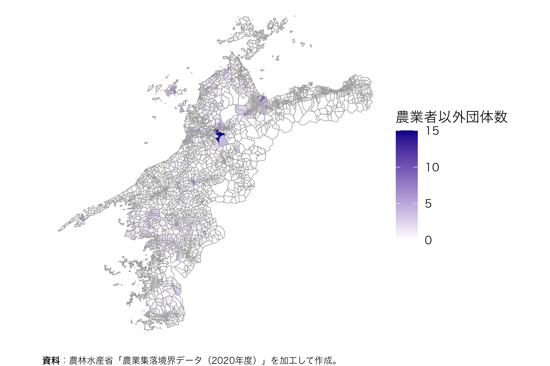
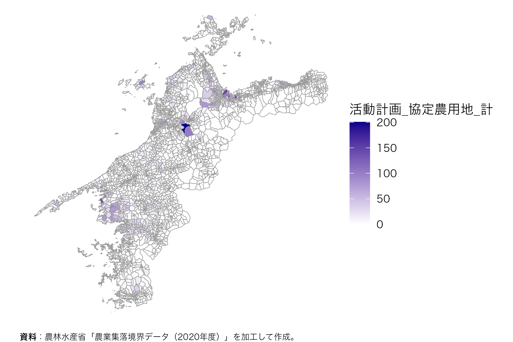
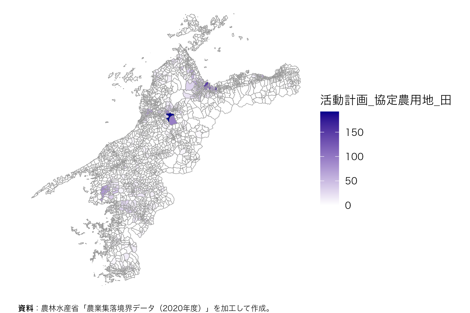
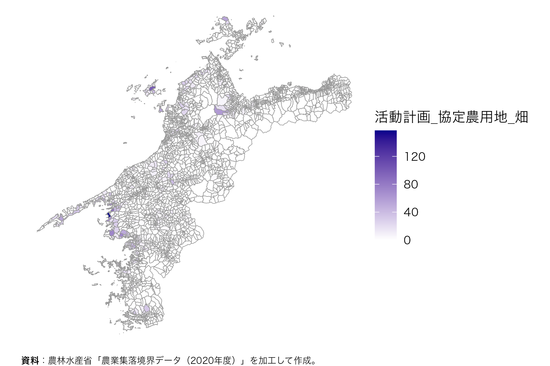
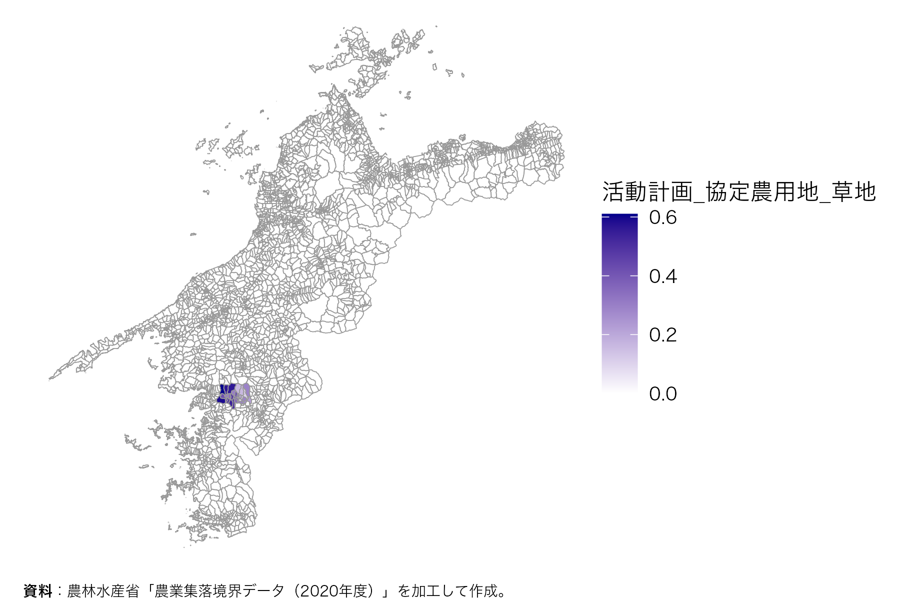
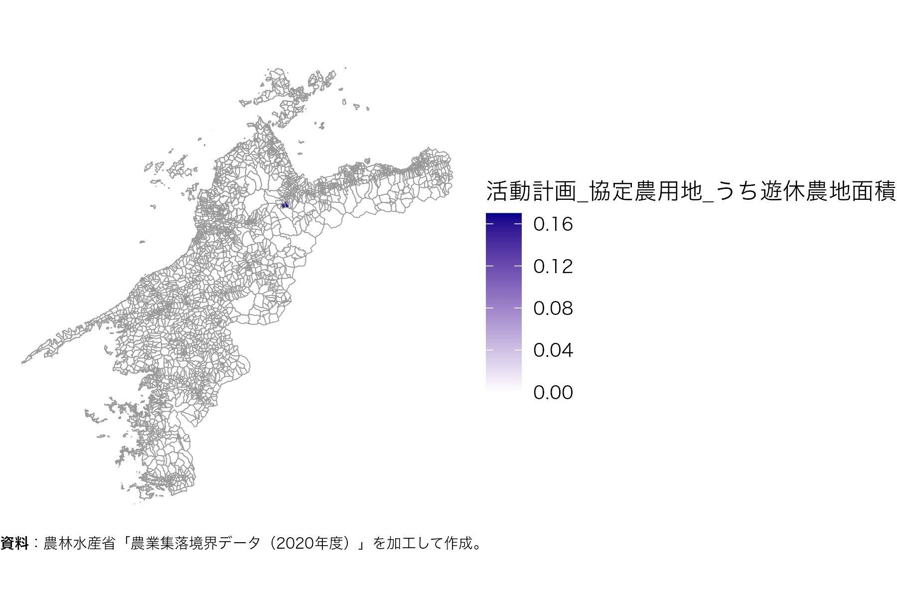
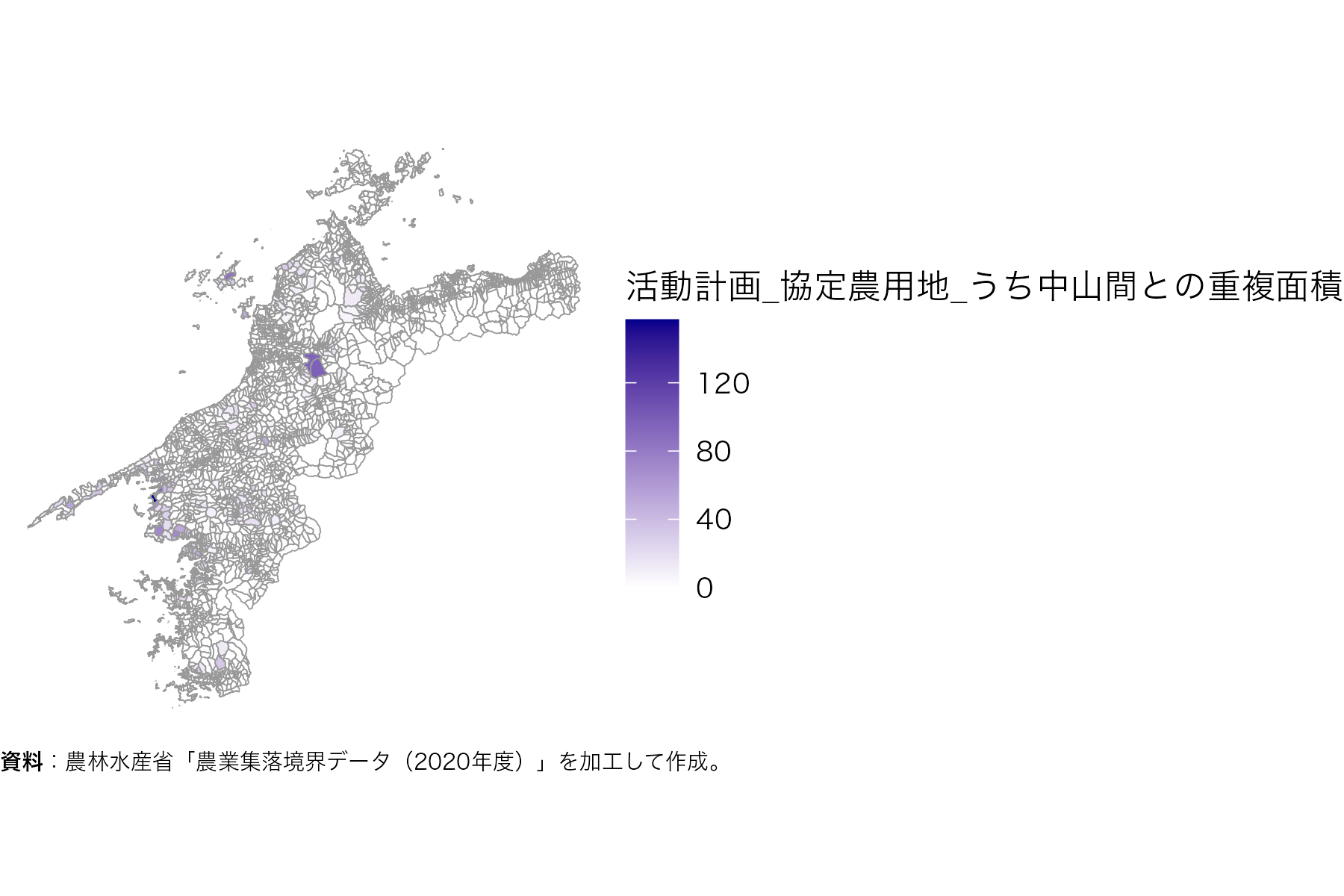
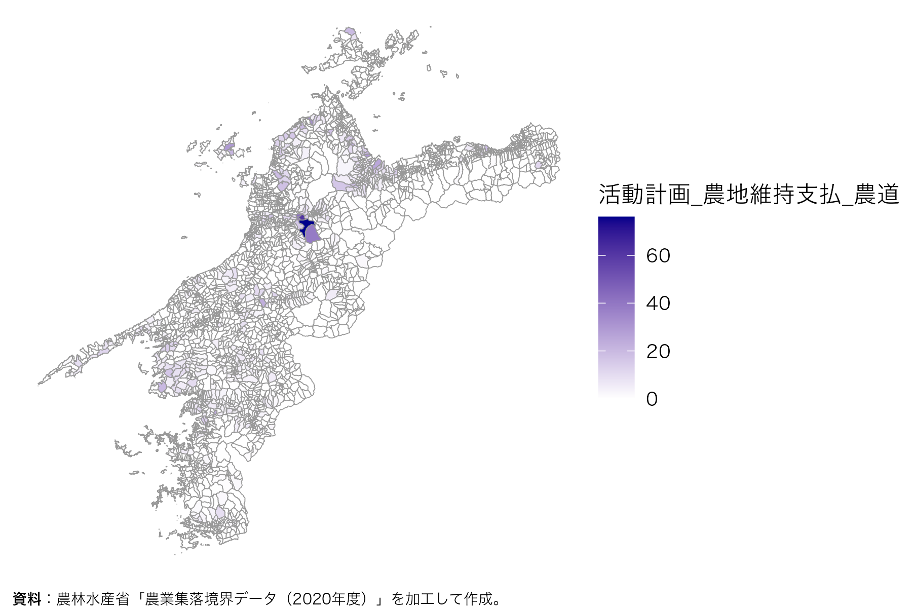
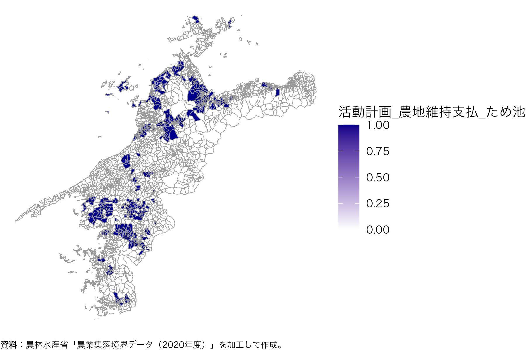
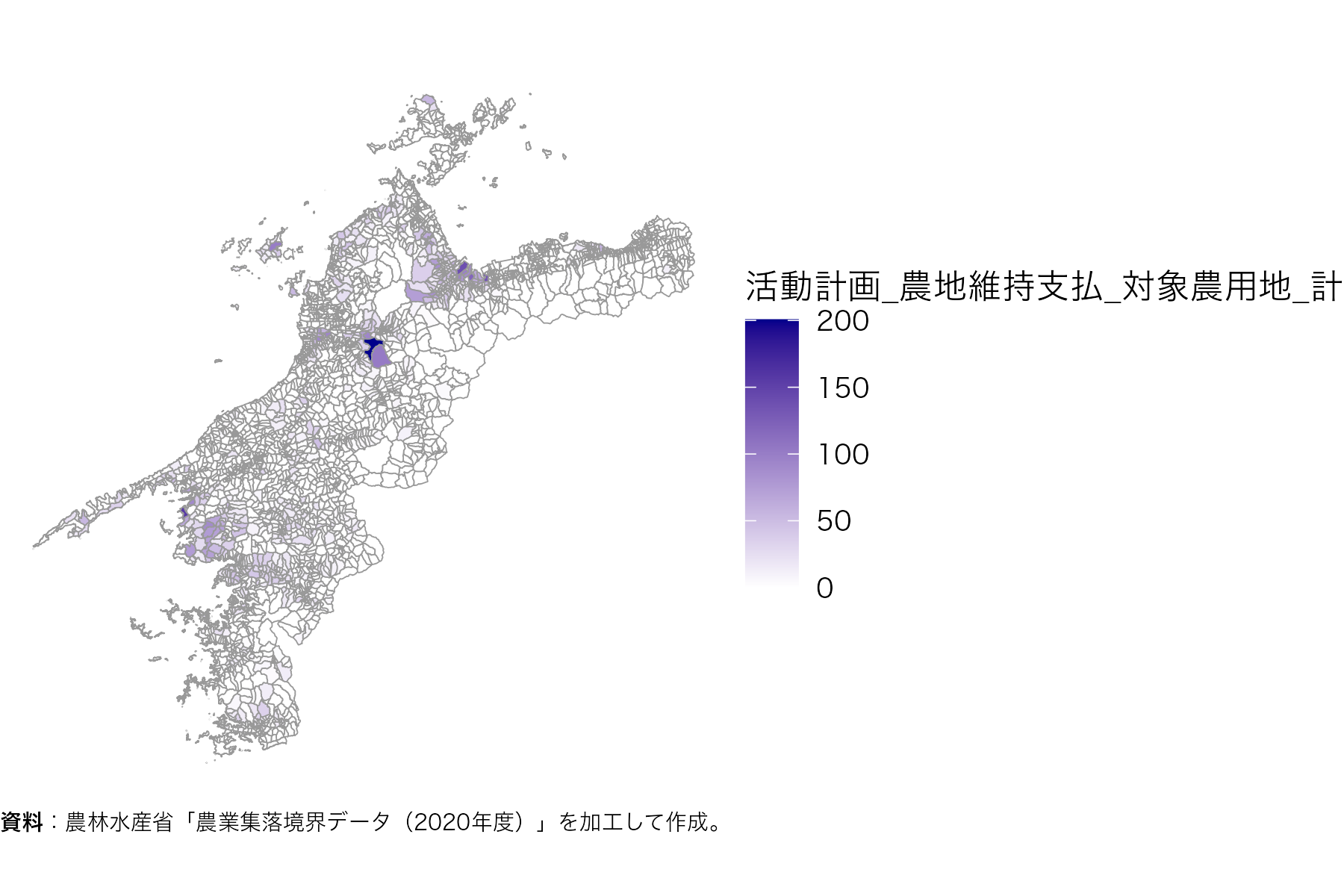
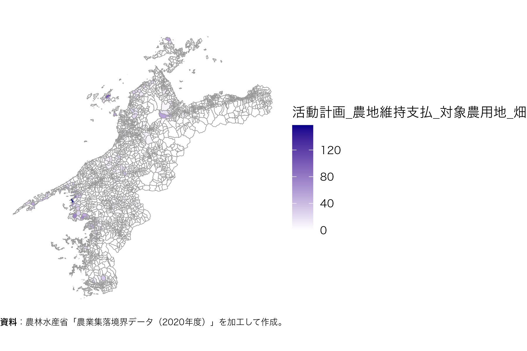
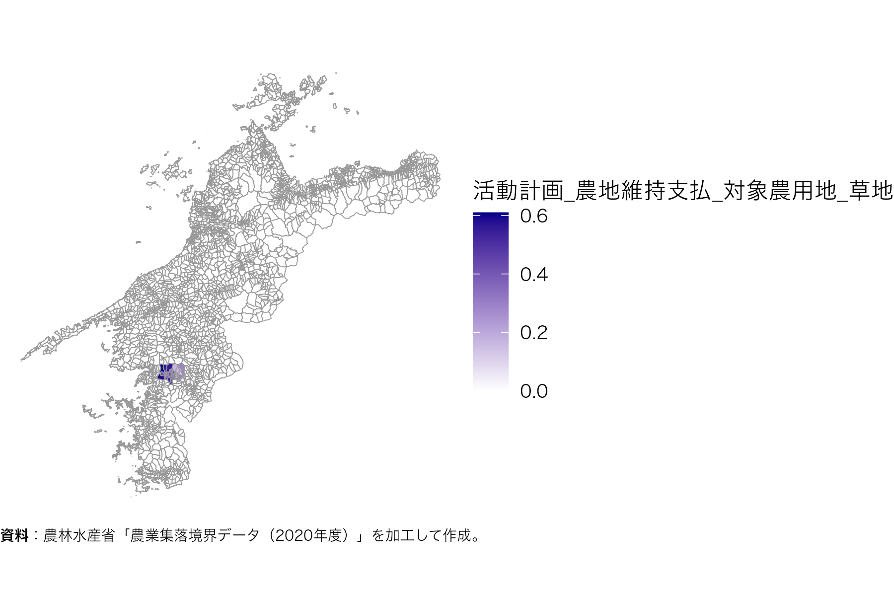
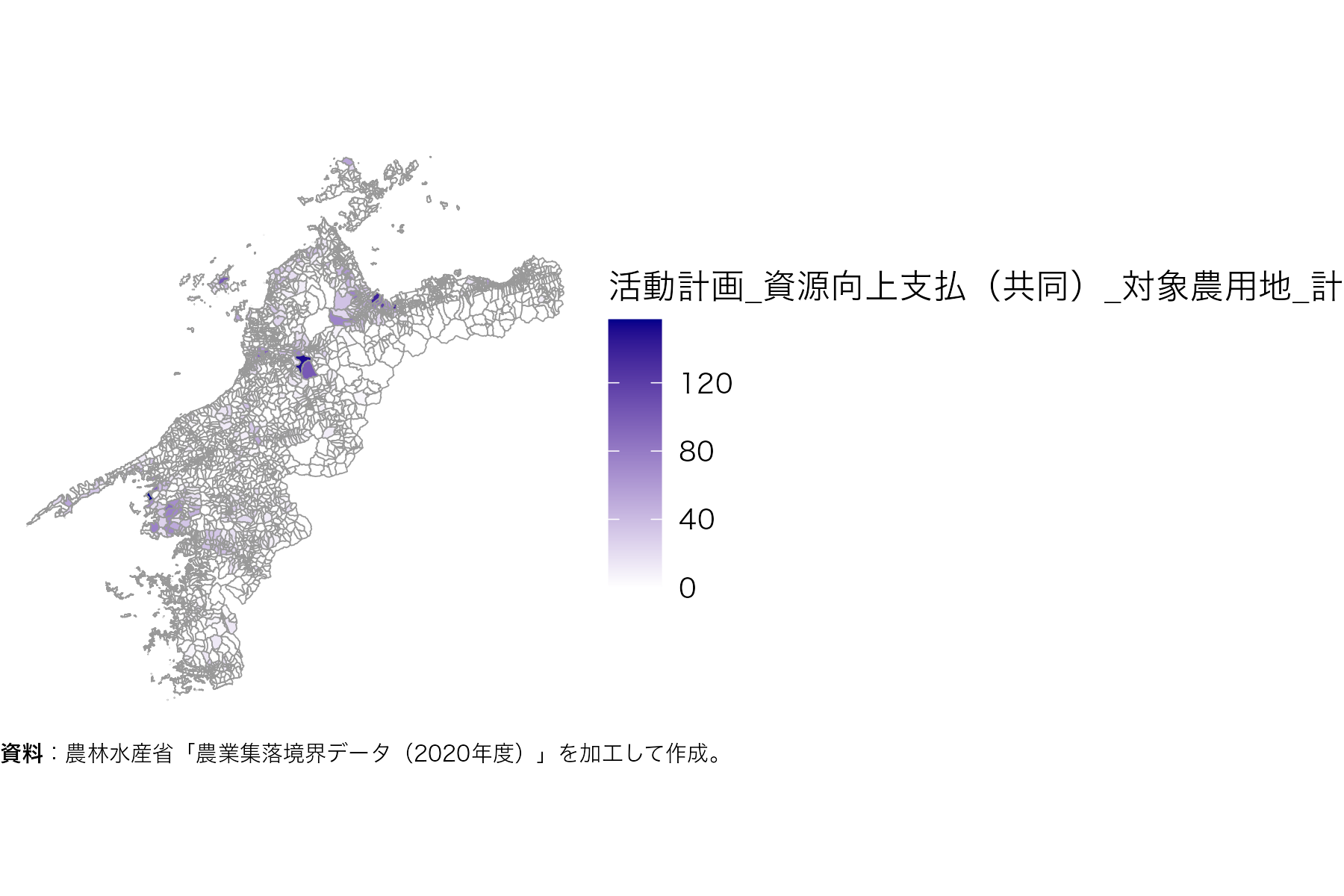
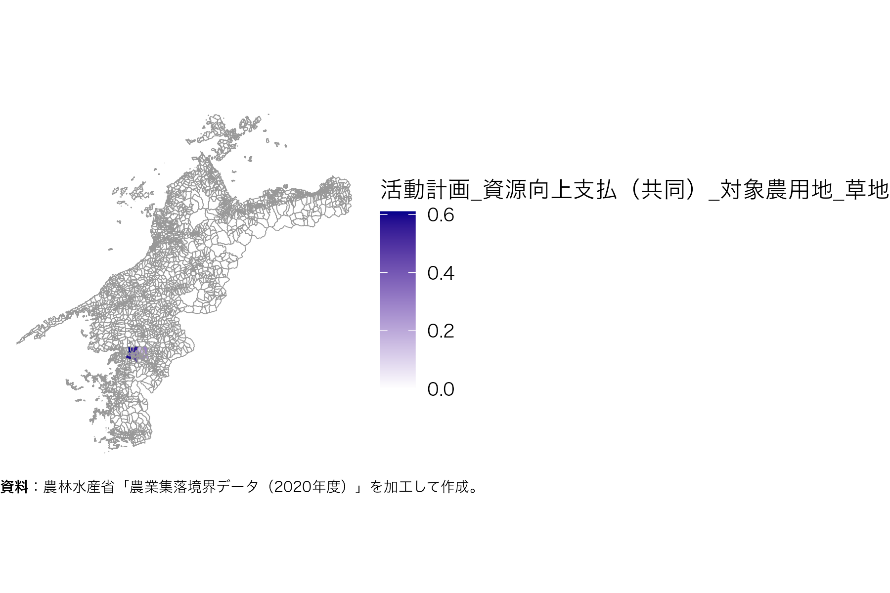
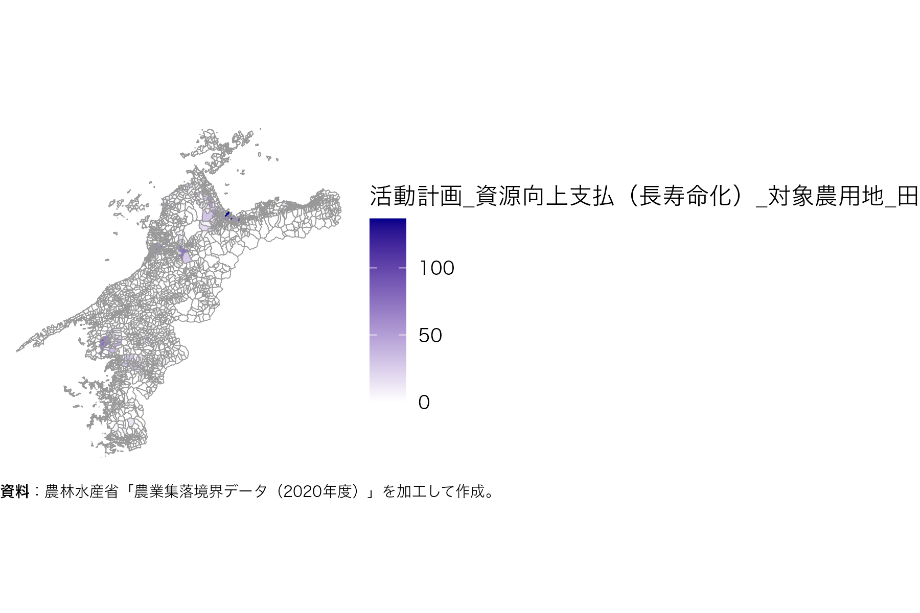
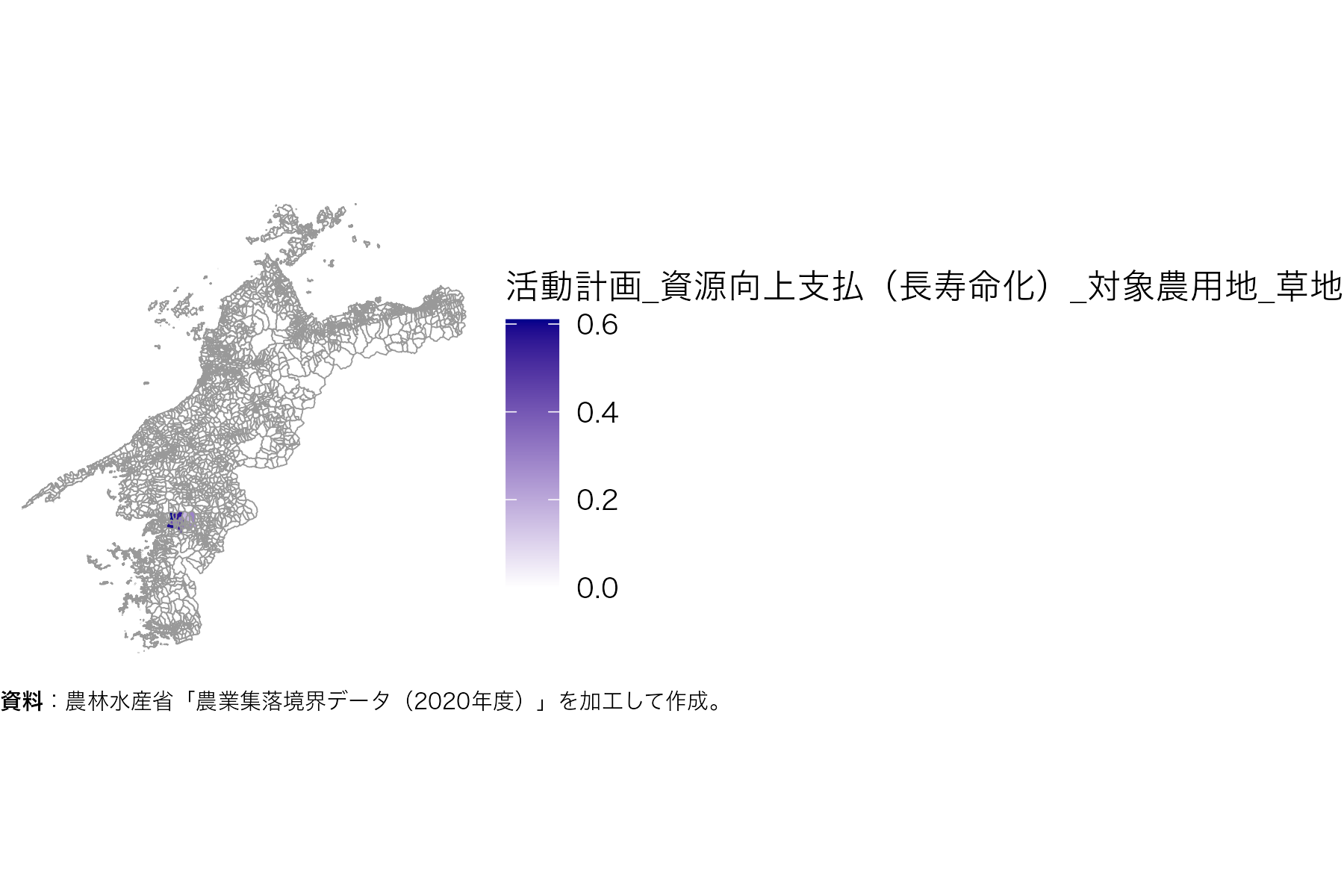
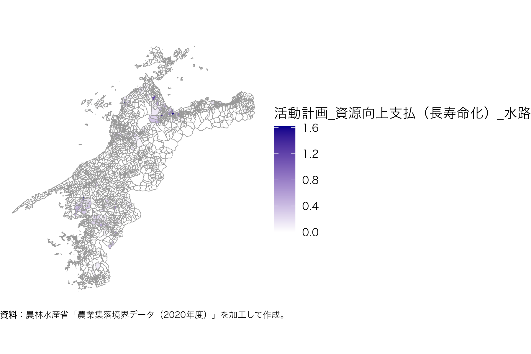
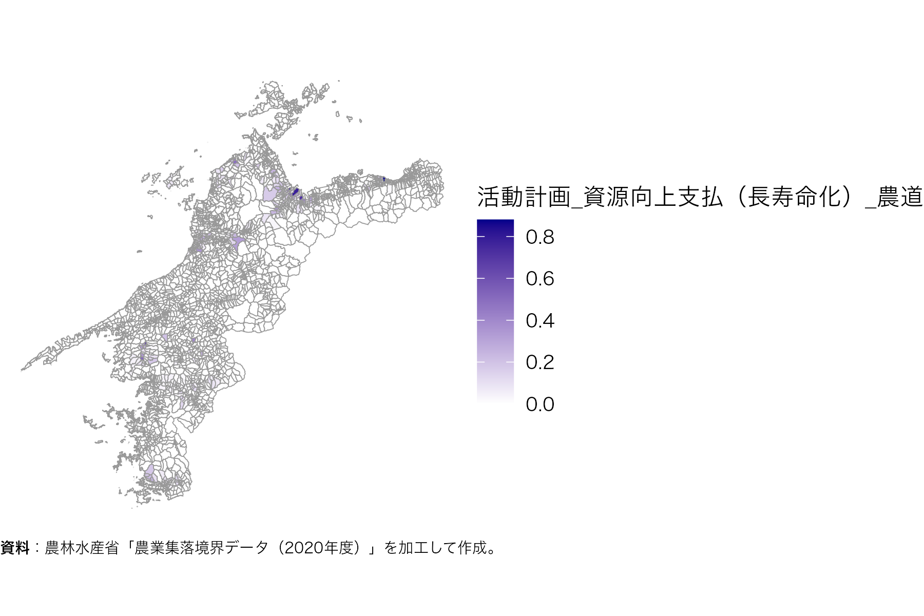
m1 <- b1 |>
  read_ikasudb("~/GC0001_2019_2020_38.xlsx")

for (i in setdiff(names(m1), names(b1[[1]]))) {
  p <- ggplot() +
    geom_sf(data = m1, aes(fill = .data[[i]]), color = "grey60") +
    scale_fill_gradient(
      low  = "white",
      high = "darkblue",
      na.value = "grey90"
    ) +
    labs(caption = paste0("**資料**：", cite_fude(m1)$ja)) +
    theme_void() +
    theme(
      plot.caption = element_markdown(size = 7, hjust = 0),
      text = element_text(family = "Hiragino Sans")
    )

  print(p)
  # ggsave(paste0(i, ".png"), p)
}