Structure of combined Fude Polygon data with agricultural community boundary data

library(fude)

d <- read_fude("~/2022_38.zip", quiet = TRUE, supplementary = TRUE)
b <- get_boundary(d, path = "~", quiet = TRUE)

d2 <- read_fude("~/MB0001_2025_2020_38.zip", quiet = TRUE)

GeoJSON data characteristics (obtain data #1)

library(sf)

db <- d |>
  lapply(st_transform, crs = 4612) |>
  combine_fude(b, city = "松山市", rcom = "由良|北浦|鷲ケ巣|門田|馬磯|泊|御手洗|船越")

There are 7 types of objects obtained by combine_fude(), as follows:

names(db)

## [1] "fude"       "fude_split" "rcom"       "rcom_union" "kcity"     
## [6] "city"       "pref"

library(ggplot2)

ggplot() +
  geom_sf(data = db$fude, aes(fill = rcom_romaji), alpha = .8) +
  guides(fill = guide_legend(reverse = TRUE, title = "Agricultural community")) +
  theme_void() +
  theme(legend.position = "bottom") +
  theme(text = element_text(family = "Hiragino Sans"))

Source: Created by processing data from the Ministry of Agriculture, Forestry and Fisheries, “Fude Polygon Data (released in FY 2022)” and “Agricultural Community Boundary Data (FY 2020)”.

Data assignment

db$fude: Automatically assigns polygons on the boundaries to a community.
db$fude_split: Provides cleaner boundaries, but polygon data near community borders may be divided.

library(patchwork)

fude <- ggplot() +
  geom_sf(data = db$fude, aes(fill = rcom_romaji), alpha = .8) +
  theme_void() +
  theme(legend.position = "none") +
  coord_sf(xlim = c(132.658, 132.678), ylim = c(33.887, 33.902))

fude_split <- ggplot() +
  geom_sf(data = db$fude_split, aes(fill = rcom_romaji), alpha = .8) +
  theme_void() +
  theme(legend.position = "none") +
  coord_sf(xlim = c(132.658, 132.678), ylim = c(33.887, 33.902))

fude + fude_split

If you need to adjust this automatic assignment, you will need to write custom code. The rows that require attention can be identified with the following command.

library(dplyr)

db$fude |>
  filter(polygon_uuid %in% (db$fude_split |> filter(duplicated(polygon_uuid)) |> pull(polygon_uuid))) |>
  st_drop_geometry() |>
  select(polygon_uuid, kcity_name, rcom_name, rcom_romaji) |>
  head()

## # A tibble: 6 × 4
##   polygon_uuid                         kcity_name rcom_name rcom_romaji
##   <chr>                                <fct>      <fct>     <fct>      
## 1 8085bc47-9af5-440f-89e9-f188d3b95746 興居島村   泊        Tomari     
## 2 26920da0-b63e-4994-a9eb-175e2982fe21 興居島村   門田      Kadota     
## 3 ac2e7293-6c2f-4feb-a95f-4729dc8d0aec 興居島村   由良      Yura       
## 4 ea130038-7035-4cf3-b71c-091783090d74 興居島村   船越      Funakoshi  
## 5 4aba8229-1b14-4eab-8a91-e10d9e841180 興居島村   船越      Funakoshi  
## 6 156a3459-25cb-494c-824f-9ba6b0fb6f23 興居島村   由良      Yura

FlatGeobuf data characteristics (obtain data #2)

The FlatGeobuf format offers a more efficient alternative to GeoJSON. A notable feature of this format is that each record already includes an accurately assigned agricultural community code.

db <- combine_fude(d2, b, city = "松山市", rcom = "由良|北浦|鷲ケ巣|門田|馬磯|泊|御手洗|船越")

ggplot() +
  geom_sf(data = db$fude, aes(fill = rcom_romaji), alpha = .8) +
  guides(fill = guide_legend(reverse = TRUE, title = "Agricultural community")) +
  theme_void() +
  theme(legend.position = "bottom") +
  theme(text = element_text(family = "Hiragino Sans"))

Source: Created by processing data from the Ministry of Agriculture, Forestry and Fisheries, “Fude Polygon Data (released in FY 2025)” and “Agricultural Community Boundary Data (FY 2020)”.

Possible values for `rcom` in `combine_fude()` and `extract_boundary()`

library(data.tree)

tree <- b[[1]] |>
  filter(grepl("松山", kcity_name)) |>
  mutate(pathString = paste(pref_name, city_name, kcity_name, rcom_name, sep = "/")) |>
  data.tree::as.Node()

tree$Do(\(x) {x$n <- if (x$isLeaf) NA_integer_ else x$count})
data.tree::SetFormat(tree, "n", \(x) if (is.na(x)) "-" else x)
print(tree, "n", limit = 30)

##                             levelName   n
## 1  愛媛県                               1
## 2   °--松山市                          1
## 3       °--松山市                    108
## 4           ¦--土居田                  -
## 5           ¦--針田                    -
## 6           ¦--小栗第１                -
## 7           ¦--小栗第２                -
## 8           ¦--小栗第３                -
## 9           ¦--藤原第１                -
## 10          ¦--藤原第２                -
## 11          ¦--竹原東                  -
## 12          ¦--竹原西                  -
## 13          ¦--生石南                  -
## 14          ¦--生石北                  -
## 15          ¦--八代                    -
## 16          ¦--南味酒                  -
## 17          ¦--南江戸                  -
## 18          ¦--朝美１                  -
## 19          ¦--朝美２                  -
## 20          ¦--朝美３                  -
## 21          ¦--宮西                    -
## 22          ¦--六軒家                  -
## 23          ¦--衣山                    -
## 24          ¦--萱町９                  -
## 25          ¦--山越                    -
## 26          ¦--姫原                    -
## 27          ¦--御幸寺                  -
## 28          ¦--本町９                  -
## 29          ¦--本町８                  -
## 30          °--... 82 nodes w/ 0 sub   -

ggplot(data = b[[1]] |> filter(grepl("松山", kcity_name))) + 
  geom_sf(fill = NA) +
  geom_sf_text(aes(label = rcom_name), size = 2, family = "Hiragino Sans") +
  theme_void()

出典：農林水産省「農業集落境界データ（2020年度）」を加工して作成。

library(collapsibleTree)

b[[1]] |>
  filter(grepl("松山", city_name)) |>
  distinct(pref_name, city_name, kcity_name, rcom_name) |>
  (\(x) collapsibleTree(
    x,
    hierarchy = names(x),
    root = "・"
  ))()

Possible values for `kcity` in `combine_fude()` and `extract_boundary()`

library(paletteer)

ggplot(b[[1]] |> filter(city_name == "松山市")) +
  geom_sf(aes(fill = kcity_name), alpha = .8) +
  theme_void() +
  theme(text = element_text(family = "Hiragino Sans")) +
  paletteer::scale_fill_paletteer_d("Polychrome::kelly")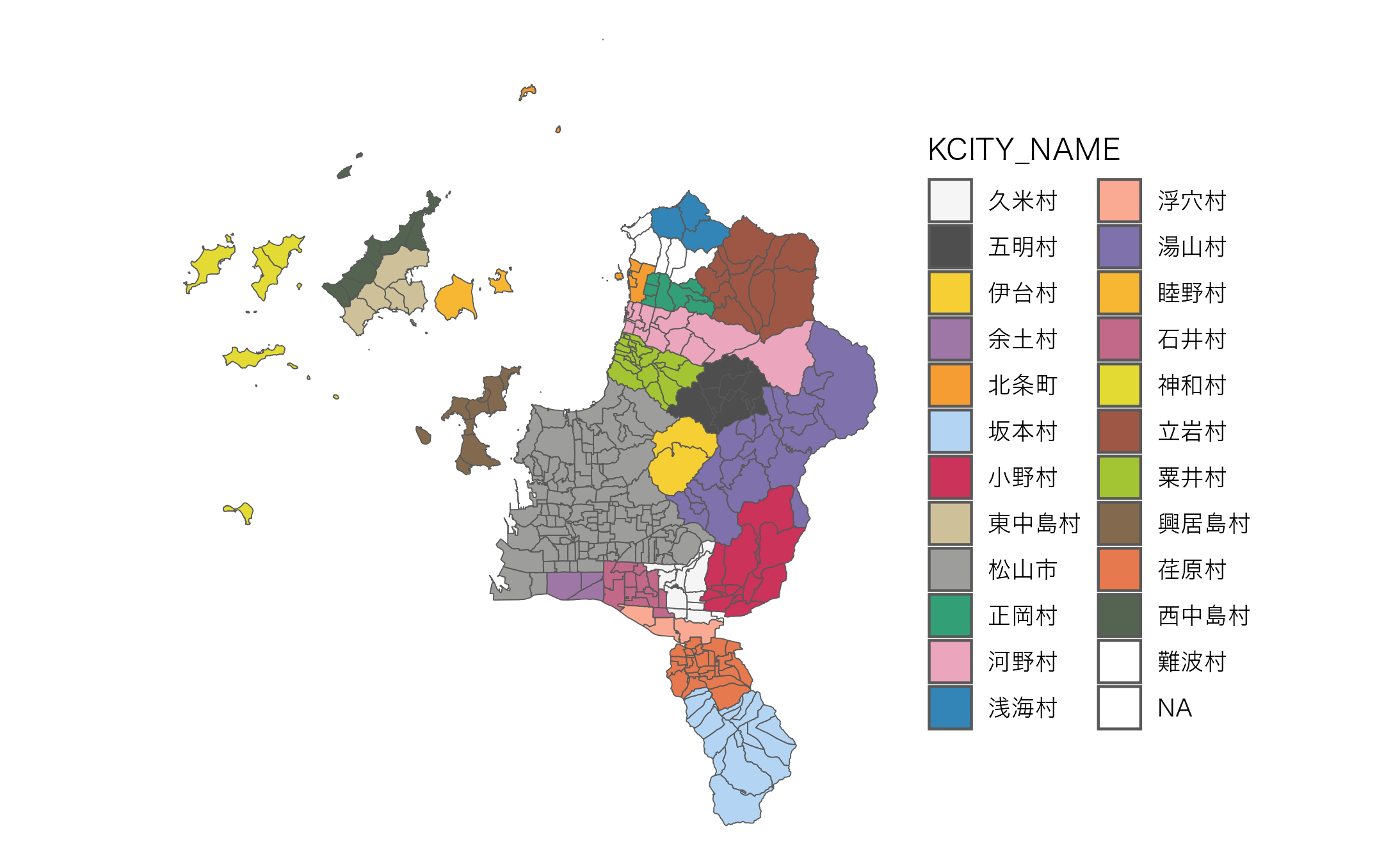

出典：農林水産省「農業集落境界データ（2020年度）」を加工して作成。

Structure of combined Fude Polygon data with agricultural community boundary data